Plot risk estimates from estimate_risk()

Generate horizontal bar charts of the risk estimates generated from estimate_risk()

Usage

plot_risk(
  risk_dat,
  add_to_dat = TRUE,
  collapse = is.data.frame(risk_dat),
  progress = TRUE,
  outcomes = "all",
  color_scheme = "single",
  color_dat = get_default_color("single"),
  color_for_last_group = get_default_color("threshold_final"),
  annotation = "all",
  legend = TRUE,
  lines = TRUE,
  line_text = TRUE,
  base_size = 12
)

Arguments

risk_dat

Data frame or list of data frames (required). This either needs to be from the output of estimate_risk()/est_risk() or needs to match the output format of estimate_risk()/est_risk(). If you wish to match the output format of estimate_risk()/est_risk(), the minimum required columns are at least one of the risk estimation columns (total_cvd, ascvd, heart_failure, chd, or stroke) and the columns over_years and model. Additionally, if you are passing a data frame of risk estimates for multiple people/instances, the preventr_id column is required to differentiate them. For each preventr_id group, there must be no more than one PREVENT model row for each possible time horizon and no more than two PCE comparison rows (one for each of the original PCEs and the revised PCEs). If preventr_id is absent from the data frame, estimation must be for a single person only, thus meaning the previously-mentioned row-composition rules apply to the full input data frame. PCE comparison rows can obviously only be for the 10-year time horizon and for the outcome of ASCVD. If you pass a list of data frames, the structure needs to be correct as well: the names of the list elements must be risk_est_10yr and risk_est_30yr, each data frame must have no more rows than there are possible models that could be run for each time horizon for a single person (i.e., 3 for 10-year risk and 1 for 30-year risk), and preventr_id must not be present in the data frames. The column input_problems is used to display a warning subtitle when estimating 30-year risk for individuals over 59 years of age; in all other cases, this column is ignored. See the vignette "plot-risk" for further discussion.

add_to_dat

Logical (optional behavior variable): Whether to add the plots as a list column to the input passed via risk_dat, either TRUE or FALSE (the default is TRUE). This argument is strict, so 1 or 0 are not accepted, and moreover, anything other than TRUE will be treated as FALSE. If TRUE, plot_risk() will return the plots in a newly-created list-column containing the plots; if FALSE, plot_risk() will return the plots directly and only the plots (no data frame component). See the vignette "plot-risk" for more information.

collapse

Logical (optional behavior variable): Whether to collapse the output into a single data frame if applicable, either TRUE or FALSE; this argument is strict, so 1 or 0 are not accepted, and moreover, anything other than TRUE will be treated as FALSE. This argument is only considered if add_to_dat is TRUE and risk_dat is a list of data frames (as happens with estimate_risk()/est_risk() when the collapse argument for that function is FALSE). This maintains consistency with the API for estimate_risk()/est_risk(). See the vignette "plot-risk" for more information.

progress

Logical (optional behavior variable): Whether to display a progress bar during execution, either TRUE (default) or FALSE. This argument is strict, so 1 or 0 are not accepted, and moreover, anything other than TRUE will be treated as FALSE. It requires the utils package, which is part of the R distribution (i.e., outside of atypical scenarios, you should not need to install the utils package yourself).

outcomes

Character (optional behavior variable): The outcome(s) to plot. This should be a character vector listing the outcomes in the order of desired plotting from top to bottom. The default of "all" gets translated internally to c("total_cvd", "ascvd", "heart_failure", "chd", "stroke"), and it overrides anything else that might be passed to outcomes.

color_scheme

Character (optional behavior variable): The color scheme to use, one of "single" (the default) or "categories". This argument is interdependent with argument color_dat.

color_dat

Character or data frame (optional behavior variable): This argument is interdependent with argument color_scheme.

• If color_scheme = "single", color_dat should be a character vector of length 1 specifying the color to use, in a format recognized by R. This includes named colors (e.g., "dodgerblue") or hexadecimal codes (e.g., "#1e90ff"). One can also specify the argument as a call to rgb() (which simply returns the hexadecimal color code as a character vector). The default is "#3c8dbc".

• If color_scheme = "categories", color_dat should be a data frame with columns threshold (numeric, 0.001 <= value <= 0.999) and color (character, adhering to specifications delineated for indicating desired color when color_scheme = "single").

  • The numeric limits keep thresholds within the range that can be displayed sensibly for proportion estimates rounded to 3 decimal places. One could, of course, easily argue even less extreme values are also not terribly sensible, either, but 0.001 and 0.999 are unequivocal simply based on how risk estimation and plotting work.

  • The data frame can have up to 3 rows specifying pairs of threshold values and corresponding colors (threshold-color pairs) to use for values below the given threshold.

  • A final threshold will always be added for values that are at or above the highest valid user-specified threshold in the data frame, and the color for this final threshold can be specified using the color_for_last_group argument.

  • Thresholds should ideally be entered in increasing order, but they can technically be entered in any order, as the function will sort them anyway.

  • The function will disregard threshold-color pairs where the threshold is empty, duplicated, or outside the aforementioned limits. The function will then sort the threshold-color pairs based on the threshold value to prevent problematic requests (e.g., threshold 1 at 0.15 and threshold 2 at 0.10 will be rearranged to 0.10 and 0.15, but the colors entered for those thresholds will be preserved during the sort). At least one valid threshold-color pair must remain after this cleaning.

  • See the "Details" section and "plot-risk" vignette for further information.

color_for_last_group

Character (optional behavior variable): The color to use for the de facto last group (i.e., values that fall at or above the highest valid user-specified threshold in the color_dat data frame). This argument is only considered when color_scheme = "categories". The default is "#dd4b39". Entry should adhere to the specifications delineated for indicating desired color when color_scheme = "single". See the "Details" section and "plot-risk" vignette as well.

annotation

Character (optional behavior variable): Whether to include all annotation ("all"), no annotation ("none"), or one or more of the components of annotation, which can be one or more of "title", "subtitle", and "caption". The default is "all". Note this does not impact the legend (where applicable).

legend

Logical (optional behavior variable): Whether to include a legend with the plot, either TRUE or FALSE (the default is TRUE). This argument is strict, so 1 or 0 are not accepted. This argument is only considered when color_scheme = "categories".

lines

Logical (optional behavior variable): Whether to include dashed vertical lines at the threshold values, either TRUE or FALSE (the default is TRUE). This argument is strict, so 1 or 0 are not accepted. This argument is only considered when color_scheme = "categories".

line_text

Logical (optional behavior variable): Whether to include caption text describing the values at which the lines are drawn (i.e., the threshold values), either TRUE or FALSE (the default is TRUE). This argument is strict, so 1 or 0 are not accepted. This argument is only considered when color_scheme = "categories" and lines = TRUE.

base_size

Numeric (optional behavior variable): The base font size to use for the plot. The default is 12. Entries that are not a single, finite, positive number will be discarded in favor of the default.

Value

An object in one of the following formats:

• a single ggplot object

• a list of ggplot objects

• a data frame with ggplots in the column plot

• a list of data frames with ggplots in the column plot

Which of these formats is returned depends on the values of the arguments add_to_dat and collapse and the structure of risk_dat. The table below summarizes the return format for various input/argument combinations:

Structure of risk_dat	Value of add_to_dat	Value of collapse	Output format
data frame	TRUE	not applicable	data frame with plot list-column
data frame	FALSE	not applicable	ggplot object or list of ggplot objects
list of data frames	TRUE	TRUE	single, collapsed data frame with plot list-column
list of data frames	TRUE	FALSE	list of data frames, each with plot list-column
list of data frames	FALSE	not applicable	list of ggplot objects

See the vignette "plot-risk" for more information and examples demonstrating these various return formats.

Details

Specifying color_dat and color_for_last_group when color_scheme = "categories"

See also the color_dat and color_scheme arguments. An example color_dat data frame might be something like the following:

 color_dat_v1 <- data.frame(
   threshold = 0.075,
   color = "#00A65A"
 )

 # or

 color_dat_v2 <- data.frame(
   threshold = c(0.075, 0.20),
   color = c("#00A65A", "#FFFDAF")
 )

 # or

 color_dat_v3 <- data.frame(
   threshold = c(0.075, 0.20, 0.35),
   color = c("#00A65A", "#FFFDAF", "#FF8C00")
 )

 # Not-great entries that will be cleaned

 color_dat_why_v1 <- data.frame(
   threshold = c(0.075, 0.20, 0.20),
   color = c("#00A65A", "#FFFDAF", "#FF8C00")
 )

 color_dat_why_v2 <- data.frame(
   threshold = c(0.35, 0.075, 1.5),
   color = c("#00A65A", "#FFFDAF", "#FF8C00")
 )

In all the above cases, users can specify color_for_last_group, and plot_risk() will automatically assign that color to values at or above the highest valid user-specified threshold. For example, suppose color_for_last_group is set as "#dd4b39" (this is also the default color for this argument). Using the above examples:

• For color_dat_v1, "#00A65A" will be applied for values below 0.075, and "#dd4b39" will be applied for values at or above 0.075.

• For color_dat_v2, "#00A65A" will be applied for values below 0.075, "#FFFDAF" will be applied for values at or above 0.075 and below 0.20, and "#dd4b39" will be applied for values at or above 0.20.

• For color_dat_v3, "#00A65A" will be applied for values below 0.075, "#FFFDAF" will be applied for values at or above 0.075 and below 0.20, "#FF8C00" will be applied for values at or above 0.20 and below 0.35, and "#dd4b39" will be applied for values at or above 0.35.

• For color_dat_why_v1, the function will clean the data frame to remove the duplicate threshold value, and the result will be the same as color_dat_v2.

• For color_dat_why_v2, the function will clean the data frame to remove the invalid threshold value of 1.5, then the thresholds will be arranged in increasing order, so the final result will be threshold 1 being at 0.075 with color "#FFFDAF", threshold 2 being at 0.35 with color "#00A65A", and the final group being at or above 0.35 with color "#dd4b39".

Examples

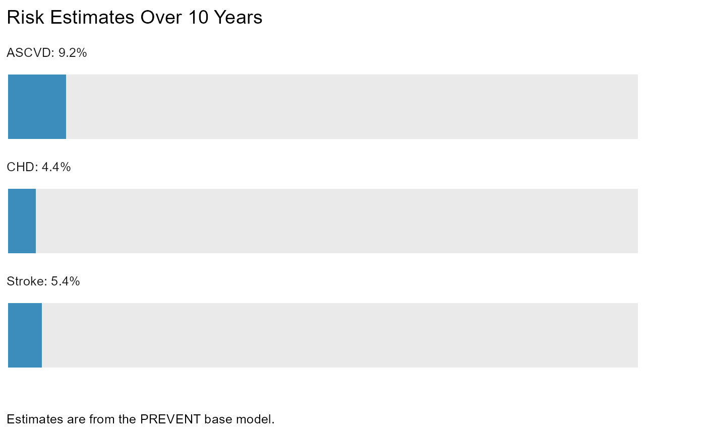
res <- estimate_risk(
  age = 50, 
  sex = "female",    
  sbp = 160, 
  bp_tx = TRUE,      
  total_c = 200,     
  hdl_c = 45,        
  statin = FALSE,    
  dm = TRUE,         
  smoking = FALSE,   
  egfr = 90,
  bmi = 35
)
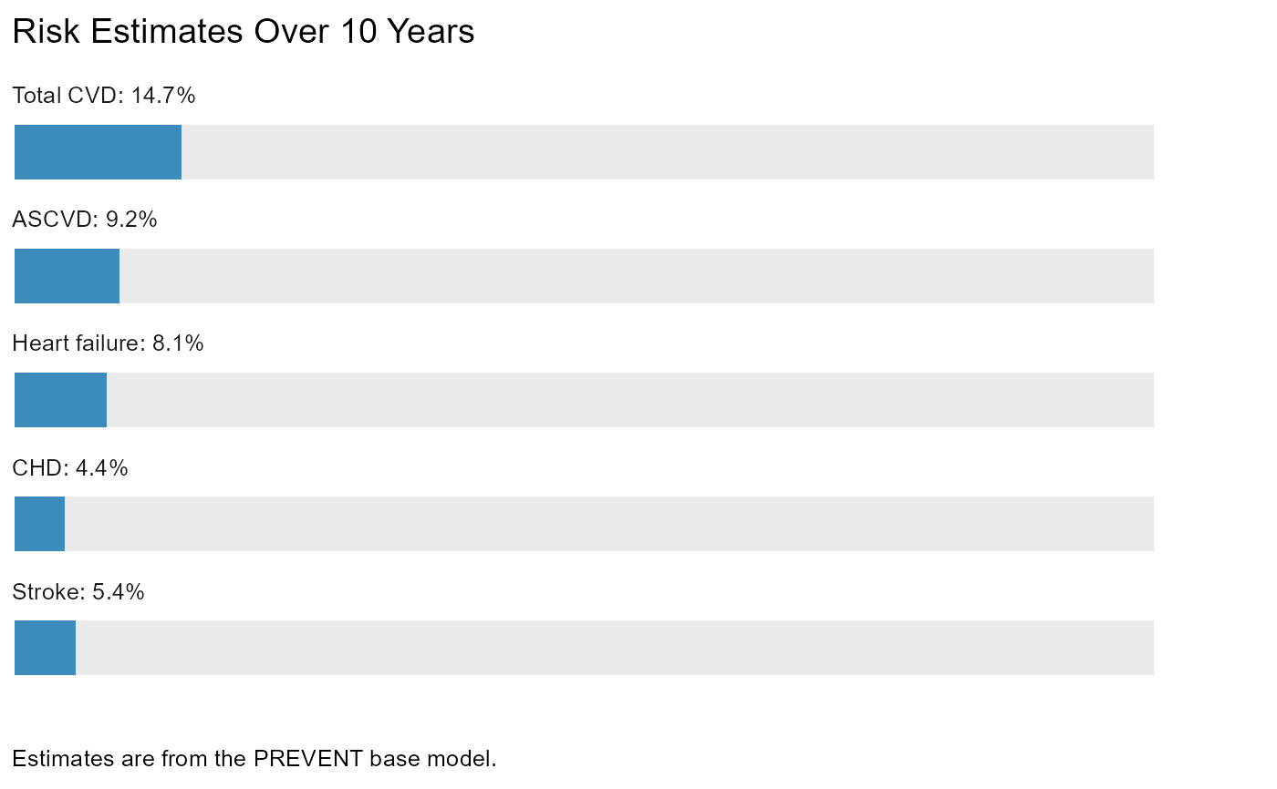
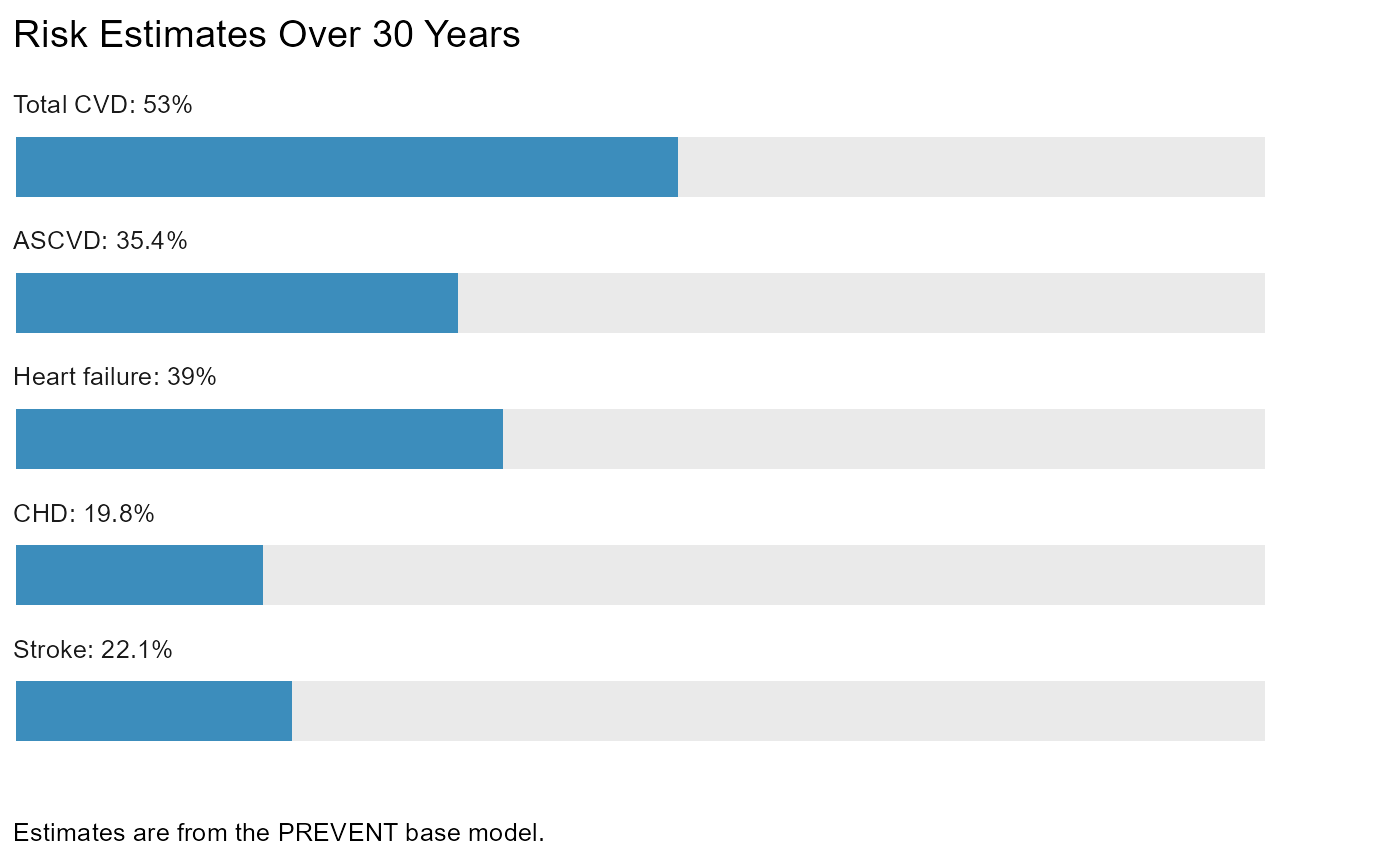
#> PREVENT estimates are from: Base model.

plot_risk(res, add_to_dat = FALSE)
#> 
  |                                                                            
  |                                                                      |   0%
  |                                                                            
  |===================================                                   |  50%
  |                                                                            
  |======================================================================| 100%
#> $risk_est_10yr

#> 
#> $risk_est_30yr

#> 

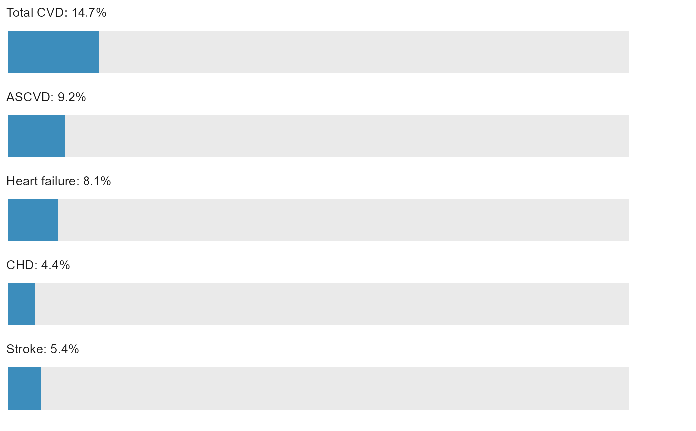
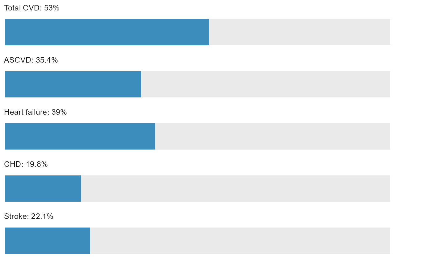
# Remove annotation
plot_risk(res, annotation = "none", add_to_dat = FALSE)
#> 
  |                                                                            
  |                                                                      |   0%
  |                                                                            
  |===================================                                   |  50%
  |                                                                            
  |======================================================================| 100%
#> $risk_est_10yr

#> 
#> $risk_est_30yr

#> 

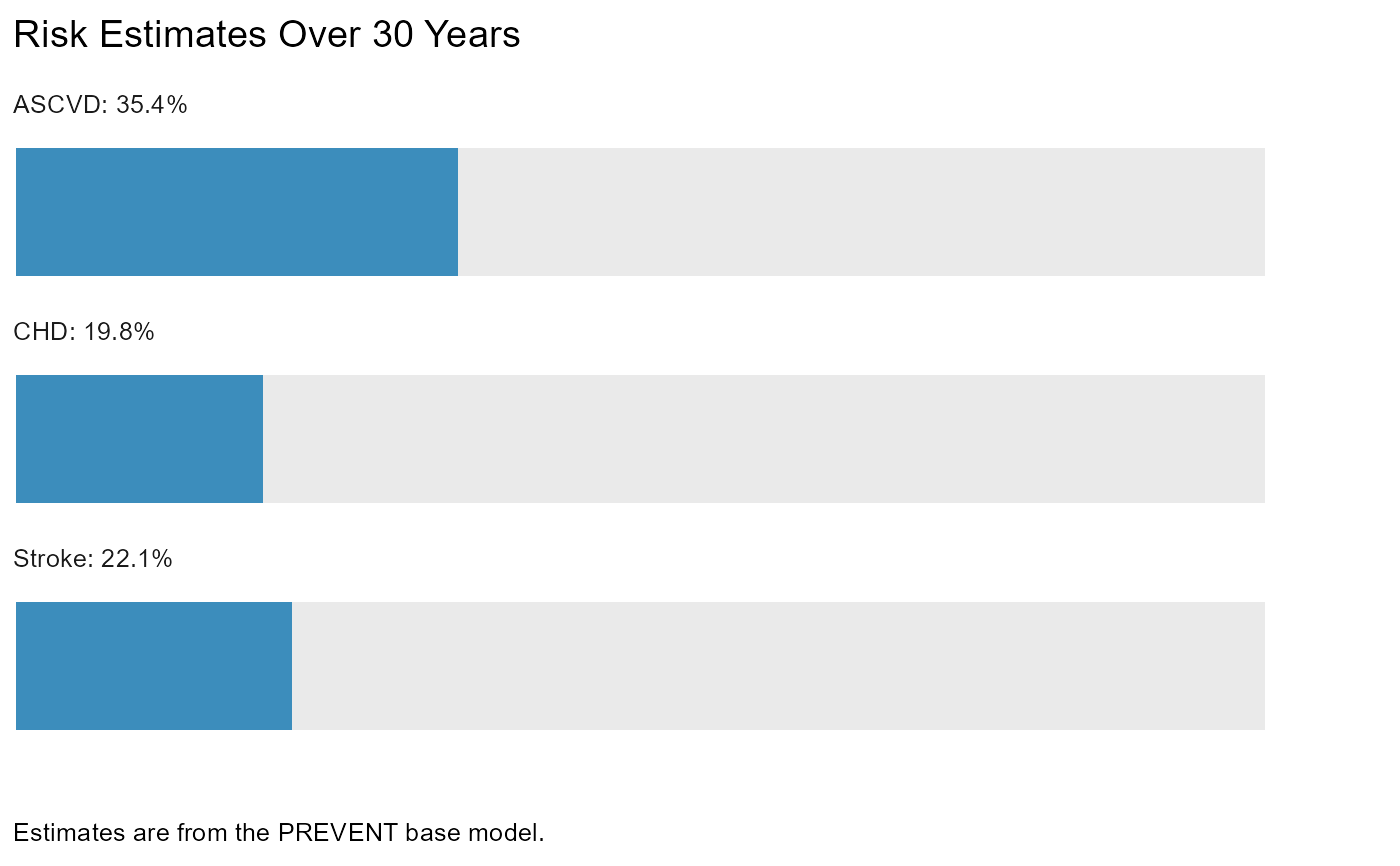
# Plot only a subset of the outcomes
# (e.g., excluding total CVD and heart failure)

plot_risk(
  res, 
  outcomes = c("ascvd", "chd", "stroke"), 
  add_to_dat = FALSE
)
#> 
  |                                                                            
  |                                                                      |   0%
  |                                                                            
  |===================================                                   |  50%
  |                                                                            
  |======================================================================| 100%
#> $risk_est_10yr

#> 
#> $risk_est_30yr

#> 

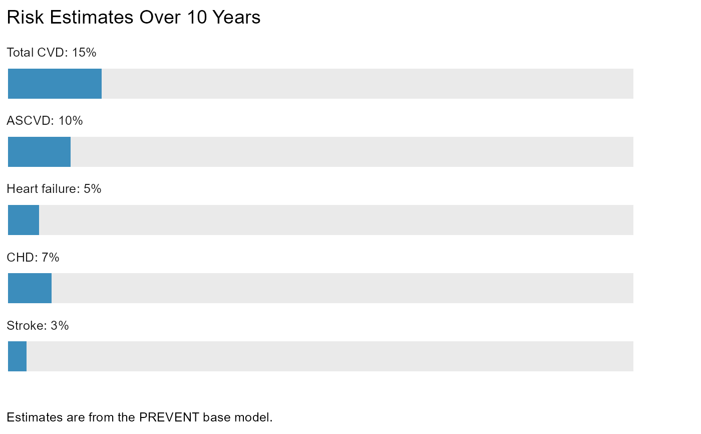
# Need to plot risk estimates you already have? No problem.
risk_dat <- data.frame(
  total_cvd = 0.15,
  ascvd = 0.10,
  heart_failure = 0.05,
  chd = 0.07,
  stroke = 0.03,
  model = "base",
  over_years = 10
)

plot_risk(risk_dat, add_to_dat = FALSE)


# Rest of examples limited to interactive sessions
if (FALSE) { # interactive()
  res_10yr <- res$risk_est_10yr
  res_30yr <- res$risk_est_30yr
  
  # Change color for `color_scheme = "single"`
  plot_risk(
    res_10yr, 
    color_scheme = "single", 
    color_dat = "darkgreen",
    add_to_dat = FALSE
  )
  
  # Use `color_scheme = "categories"`
  color_dat <- data.frame(
    threshold = c(0.075, 0.20),
    color = c("#00A65A", "#FF8C00")
  )
   
  plot_risk(
    res_30yr, 
    color_scheme = "categories", 
    color_dat = color_dat,
    add_to_dat = FALSE
  )
  
  # Change color for final group
  plot_risk(
    res_30yr, 
    color_scheme = "categories", 
    color_dat = color_dat,
    color_for_last_group = "maroon",
    add_to_dat = FALSE
  )
  
  # Remove legend
  plot_risk(
    res_10yr,
    color_scheme = "categories",
    color_dat = color_dat,
    legend = FALSE,
    add_to_dat = FALSE
  )
  
  # Remove legend and lines
  plot_risk(
    res_10yr,
    color_scheme = "categories",
    color_dat = color_dat,
    legend = FALSE,
    lines = FALSE,
    add_to_dat = FALSE
  )
  
  # Remove legend and line text (but keep lines)
  plot_risk(
   res_10yr,
   color_scheme = "categories",
   color_dat = color_dat,
   legend = FALSE,
   line_text = FALSE,
   add_to_dat = FALSE
  )
  
  # Run `plot_risk()` on a data frame of results from 
  # `estimate_risk()`/`est_risk()`   
  dat <- data.frame(
    age = c(40, 50, 60), 
    sex = c("female", "female", "male"),    
    sbp = c(160, 120, 140),
    bp_tx = c(TRUE, TRUE, FALSE),     
    total_c = c(200, 189, 156),    
    hdl_c = c(45, 42, 38),       
    statin = c(FALSE, TRUE, TRUE),   
    dm = c(TRUE, FALSE, TRUE),       
    smoking = c(FALSE, TRUE, FALSE),  
    egfr = c(90, 85, 88),
    bmi = c(35, 22, 28)
  )
  
  res <- estimate_risk(use_dat = dat)

  plot_risk(res, add_to_dat = FALSE) # Returns plots

  plot_risk(res) # Returns data frame `plot` list-column

  # Because the plots are ggplot objects, they can be further customized
  # like any other ggplot object.
  res_10yr <- estimate_risk(use_dat = dat[1, ], time = 10)
  # Customization via {ggplot2}
  p <- plot_risk(res_10yr, add_to_dat = FALSE)
  # Note `labs()`, `theme()`, and `margin()` are from {ggplot2}, so one would
  # need to get access to them via, e.g., `library(ggplot2)`, `ggplot2::` prefixing, 
  # `importFrom()` (if developing a package; for example, {preventr} `importFrom()`s
  # all three), etc. 
  p + 
    ggplot2::labs(title = "Lorem ipsum") + 
    ggplot2::theme(plot.margin = ggplot2::margin(20, 20, 20, 20))
  # etc.
  # It is also easy to combine the 10- and 30-year plots if desired, e.g., 
  # via packages like {patchwork} with functions like `patchwork::wrap_plots()`,
  # and there are many additional options for composing plots via {patchwork}.
}